


 Categories
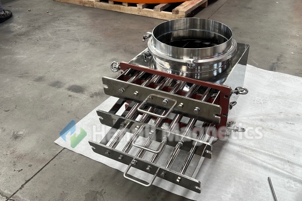
What separates an ordinary magnetic grate separators from a high-performance one? The answer lies not in the number of magnetic rod elements, but in how they are arranged. A few millimeters of spacing, a shift in polarity, or a change in layering can determine whether a magnetic rod array captures every last ferrous particle or lets contamination slip through. For decades, this arrangement was guided by experience and trial-and-error. Today, magnetic field simulation has transformed the design of magnetic grate separators from an art into a precise science.
The Three Contradictions of Magnetic Rod Arrays
Every magnetic rod layout must balance competing demands:
-
Field Strength vs. Uniformity: Strong magnetic fields are essential for capture, but poorly arranged magnetic rod elements can create concentrated zones of high intensity while leaving flow channels with weak fields—blind spots where particles escape.
-
Efficiency vs. Capacity: Dense magnetic rod arrays capture more contaminants but increase flow resistance and clogging risk.
-
Upstream vs. Downstream Capture: The first magnetic rod in the flow path captures the most particles. But if it becomes saturated, it can magnetically shield downstream rods, dramatically reducing overall magnetic grate separators performance.
 The Simulation Workflow: From Virtual Model to Optimized Design
Magnetic simulation software solves Maxwell’s equations across a three-dimensional model, revealing what cannot be seen with the naked eye.
Step One: Build the Virtual Model
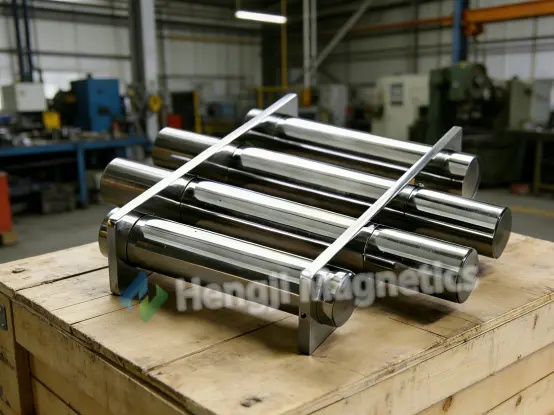
The engineer creates an exact digital replica of the magnetic rod array, including the stainless steel tubes, housing, and the fluid or air space where material flows. Material properties—the BH curve of the Neodymium magnets, the permeability of the stainless steel—are precisely defined.
Step Two: Define and Solve
Each magnetic rod is assigned a magnetization direction. The simulation then calculates the magnetic field strength and flux density at every point in the space around the array.
Step Three: Visualize and Quantify
The software produces visual maps that reveal the hidden behavior of the magnetic grate separators:
-
Field Strength Contours: Color-coded maps show exactly where the magnetic field is strong and where it is weak. The goal is uniform, high-strength coverage across the entire flow cross-section.
-
Magnetic Force Vectors: Arrows show the direction of magnetic force, ensuring it points toward the magnetic rod surfaces where capture occurs.
-
Field Line Distribution: Dense field lines crossing the flow path indicate efficient use of magnetic flux.
-
Path Profiles: Engineers can plot field strength along the centerline of the flow channel, identifying any gaps where the field drops below the capture threshold.
 Optimizing the Array with Simulation Data
With these visual insights, engineers can systematically refine the magnetic rod arrangement.
Spacing and Layer Optimization
-
The Question: How far apart should magnetic rod elements be placed? Too close wastes material and restricts flow; too far creates capture gaps.
-
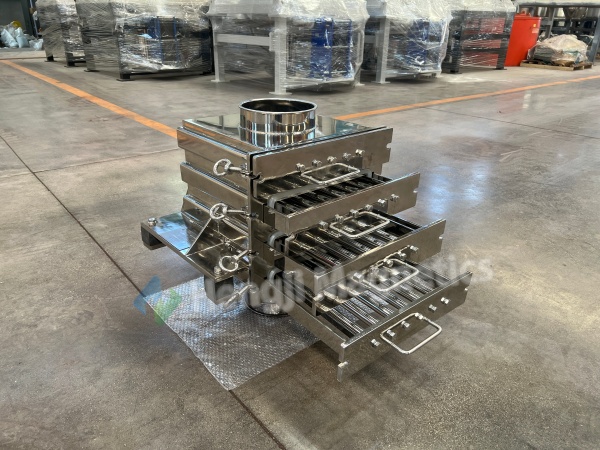
The Simulation Answer: Run multiple simulations with different spacings, identify the minimum field strength between rods, and select the spacing that maintains capture-grade fields across the entire gap. For multi-layer magnetic grate separators, simulate the interaction between layers to find the optimal distance that balances capture efficiency with flow capacity.
Magnetization Direction and Layout Pattern
-
Axial vs. Radial Magnetization: Simulating both reveals that radially magnetized magnetic rod elements produce a more uniform cylindrical field, ideal for pipeline installations.
-
Aligned vs. Staggered Grids: Staggered arrays consistently show more uniform field coverage with fewer blind spots than simple aligned grids.
Polarity Arrays: The Hidden Secret
The most advanced magnetic grate separators use alternating polarities—north and south-facing rods interleaved. Simulation reveals that this arrangement creates extreme magnetic gradients in the spaces between magnetic rod elements. For micron-sized, weakly magnetic particles, these gradients generate the intense local forces required for capture.
Mitigating Magnetic Shielding
-
The Problem: As the upstream magnetic rod captures ferrous particles, it becomes a magnetized mass that shields downstream rods.
-
The Simulation Solution: Models can simulate the array with a layer of captured iron on the first rods, quantifying the field attenuation downstream. This data guides decisions on rod spacing, gradient compensation, or optimal cleaning frequency to maintain performance.
Why Simulation Changes Everything
-
From Guesswork to Certainty: Performance can be predicted before a single prototype is built.
-
Customized for Your Material: Viscosity, flow rate, and particle size can be factored into the simulation to create a magnetic rod layout optimized for specific applications.
-
Visualizing the Invisible: Weak spots in the magnetic grate separators become visible, guiding targeted improvements like adding flux concentrators or reshaping housing elements.
-
Cost-Effective Design: Simulations identify the minimum number of magnetic rod elements required to meet performance targets, reducing material costs without compromising efficiency.
Conclusion: Engineering the Perfect Magnetic Trap
The secret of magnetic rod arrays is no longer a guarded trade secret. It is a field of engineering made visible through simulation. With powerful software tools, designers can see the invisible magnetic field, measure its strength at every point, and strategically position each magnetic rod to create an array with optimized strength, gradient, coverage, and longevity. The result is a magnetic grate separators that captures more contaminants, handles higher flow rates, and requires less frequent cleaning—all achieved through the science of magnetic field optimization.


